Lifespan of an NBA Player

Data Loading

Looking at the lifespan of an NBA player. The first thing is to load the data for each player into the workspace and get and understanding of its contents. I will try to make this data available but I am in the middle of determining which of multiple sources is the most robust and the cleanest, so I have multiple versions with various differences. The head and str functions are used to get a representation of what the data looks like.

library(plyr)
library(survival)

## Loading required package: splines

# Load data
load("~/Desktop/r/hoops/player_detail.RData")

str(player)

## 'data.frame':    21247 obs. of  9 variables:
##  $ name   : chr  "Alaa Abdelnaby" "Alaa Abdelnaby" "Alaa Abdelnaby" "Alaa Abdelnaby" ...
##  $ positon: chr  "F" "F" "F" "F" ...
##  $ Age    : num  22 23 24 24 25 26 26 22 23 24 ...
##  $ Team   : chr  "POR" "POR" "MIL" "BOS" ...
##  $ G      : num  43 71 12 63 13 3 51 82 82 81 ...
##  $ Min    : chr  "290" "934" "159" "1152" ...
##  $ Pts    : chr  "135" "432" "64" "514" ...
##  $ PPG    : chr  "3.1" "6.1" "5.3" "8.2" ...
##  $ Season : num  1990 1991 1992 1992 1993 ...

head(player)

##             name positon Age Team  G  Min Pts PPG Season
## 1 Alaa Abdelnaby       F  22  POR 43  290 135 3.1   1990
## 2 Alaa Abdelnaby       F  23  POR 71  934 432 6.1   1991
## 3 Alaa Abdelnaby       F  24  MIL 12  159  64 5.3   1992
## 4 Alaa Abdelnaby       F  24  BOS 63 1152 514 8.2   1992
## 5 Alaa Abdelnaby       F  25  BOS 13  159  64 4.9   1993
## 6 Alaa Abdelnaby       F  26  PHI  3   30   2 0.7   1994

Data Creation

The next step would typically be cleaning. I have already done lots of cleaning to this data to get it the stage that it is at though. Maybe that will be another post. The step after cleaning is often using the raw data to create variables of interest for the analytics task at hand. For survival analysis it is necessary to have variables that describe the lifespan of players as well as when they started. Next we will aggregate some of the raw data down into a more tidy format, one row per player as opposed to one row per player per season per team, how the source is formatted.

# Before we can start grouping rows by player we need a unique identifier.
# Players may have a common name, so lets create a manner to step 
# around that. 
player$bday <- player$Season - player$Age
puid <- unique(player[, c('name', 'bday')])
puid$guid <- 1:nrow(puid)
player <- merge(player, puid)
head(player)

##         name bday positon Age Team  G  Min  Pts  PPG Season guid
## 1 A.c. Green 1963       F  22  LAL 82 1542  521  6.4   1985 1320
## 2 A.c. Green 1963       F  23  LAL 79 2240  852 10.8   1986 1320
## 3 A.c. Green 1963       F  24  LAL 82 2636  937 11.4   1987 1320
## 4 A.c. Green 1963       F  25  LAL 82 2510 1088 13.3   1988 1320
## 5 A.c. Green 1963       F  26  LAL 82 2709 1061 12.9   1989 1320
## 6 A.c. Green 1963       F  27  LAL 82 2164  750  9.1   1990 1320

# Need to do some data aggrations to create some needed varaibles.

# How long a player lasted in the NBA.
span <- ddply(player, .(guid), summarise, span = max(Age) - min(Age))
head(span)

##   guid span
## 1    1    4
## 2    2   19
## 3    3   28
## 4    4    5
## 5    5   11
## 6    6    4

# A players first season
rookie <- ddply(player, .(guid), summarise, rookie = min(Season))
head(rookie)

##   guid rookie
## 1    1   1990
## 2    2   1969
## 3    3   1972
## 4    4   1997
## 5    5   1996
## 6    6   1976

# The number of games a player played there first year.
games <- ddply(player, .(guid), summarise, games = sum(G))
head(games)

##   guid games
## 1    1   256
## 2    2  1560
## 3    3   641
## 4    4   236
## 5    5   830
## 6    6   319

# Join these data sets together to form one data set.
res <- unique(player[c('name', 'positon', 'guid')])
res <- merge(res, rookie, by = 'guid')
res <- merge(res, span, by = 'guid')
res <- merge(res, games, by = 'guid')

# Cleanup the workspace
rm(span, rookie, games, puid, player)

head(res)

##   guid                name positon rookie span games
## 1    1      Alaa Abdelnaby       F   1990    4   256
## 2    2 Kareem Abdul-jabbar       C   1969   19  1560
## 3    3    Mahmo Abdul-rauf       G   1972   28   641
## 4    4   Tariq Abdul-wahad       G   1997    5   236
## 5    5 Shareef Abdur-rahim       F   1996   11   830
## 6    6       Tom Abernethy       F   1976    4   319

Data Cleanup

This is now starting to look like tidy data. We have one row per player, along with how long they played, the first year they played and two descriptive variables about their fist season.

We will still push this further. Just a few nit picky things as well as creating some variables to answer a few questions later on. Also we need to think about what to do about players that are still playing?

# The count is off by one.
res$span <- res$span + 1

# Average games per season
res$avgGam <- res$games / res$span

# Do you play a lot of games, binary
res$gamBin <- ifelse(res$avgGam > 50, 'a', 'b')

# Clean up data frame.
res$games <- NULL

# A few players have no age in the data
res <- res[complete.cases(res), ]

# Order by players with a longer history
res <- res[order(res$span, decreasing = T), ]

# Create the year they retired
res$retire <- res$span + res$rookie

# If that's before 2014 they retired, otherwise the data is censored in time. 
res$event <- ifelse(res$retire < 2014, 1, 0)

Survival Analysis

The data is now ready to run a survival analysis. We can run one with a constant to determine the most likely lifespans.

kms <- survfit(Surv(res$span, res$event) ~ 1)
summary(kms)

## Call: survfit(formula = Surv(res$span, res$event) ~ 1)
## 
##  time n.risk n.event survival  std.err lower 95% CI upper 95% CI
##     1   3964    1178 0.702825 0.007259     6.89e-01      0.71720
##     2   2786     484 0.580727 0.007837     5.66e-01      0.59629
##     3   2302     354 0.491423 0.007940     4.76e-01      0.50723
##     4   1948     273 0.422553 0.007846     4.07e-01      0.43821
##     5   1675     212 0.369072 0.007664     3.54e-01      0.38440
##     6   1463     197 0.319374 0.007405     3.05e-01      0.33422
##     7   1266     174 0.275479 0.007096     2.62e-01      0.28974
##     8   1092     178 0.230575 0.006690     2.18e-01      0.24407
##     9    914     149 0.192987 0.006268     1.81e-01      0.20567
##    10    765     180 0.147578 0.005633     1.37e-01      0.15904
##    11    585     149 0.109990 0.004969     1.01e-01      0.12017
##    12    436     121 0.079465 0.004296     7.15e-02      0.08835
##    13    315     107 0.052472 0.003542     4.60e-02      0.05989
##    14    208      74 0.033804 0.002870     2.86e-02      0.03993
##    15    134      55 0.019929 0.002220     1.60e-02      0.02479
##    16     79      30 0.012361 0.001755     9.36e-03      0.01633
##    17     49      25 0.006054 0.001232     4.06e-03      0.00902
##    18     24      10 0.003532 0.000942     2.09e-03      0.00596
##    19     14       8 0.001514 0.000617     6.80e-04      0.00337
##    20      6       2 0.001009 0.000504     3.79e-04      0.00269
##    21      4       2 0.000505 0.000357     1.26e-04      0.00202
##    23      2       1 0.000252 0.000252     3.55e-05      0.00179
##    29      1       1 0.000000      NaN           NA           NA

plot(kms, xlab = 'Seasons', ylab = 'Survival Probability')

This is pretty interesting, there is a big drop off in the first year. This seems plan out, thus experience is good. That sounds a bit odd though. Lets add a players position to see if they are all similar.

kms <- survfit(Surv(res$span, res$event) ~ res$positon)
summary(kms)

## Call: survfit(formula = Surv(res$span, res$event) ~ res$positon)
## 
##                 res$positon=C 
##  time n.risk n.event survival std.err lower 95% CI upper 95% CI
##     1    635     151  0.76220 0.01689     0.729801       0.7960
##     2    484      79  0.63780 0.01907     0.601486       0.6763
##     3    405      62  0.54016 0.01978     0.502752       0.5803
##     4    343      32  0.48976 0.01984     0.452386       0.5302
##     5    311      31  0.44094 0.01970     0.403970       0.4813
##     6    280      36  0.38425 0.01930     0.348222       0.4240
##     7    244      31  0.33543 0.01874     0.300649       0.3742
##     8    213      31  0.28661 0.01794     0.253516       0.3240
##     9    182      26  0.24567 0.01708     0.214368       0.2815
##    10    156      37  0.18740 0.01549     0.159380       0.2203
##    11    119      27  0.14488 0.01397     0.119936       0.1750
##    12     92      26  0.10394 0.01211     0.082716       0.1306
##    13     66      18  0.07559 0.01049     0.057589       0.0992
##    14     48      14  0.05354 0.00893     0.038609       0.0743
##    15     34      13  0.03307 0.00710     0.021717       0.0504
##    16     21       5  0.02520 0.00622     0.015533       0.0409
##    17     16       6  0.01575 0.00494     0.008515       0.0291
##    18     10       5  0.00787 0.00351     0.003289       0.0189
##    19      5       2  0.00472 0.00272     0.001528       0.0146
##    20      3       1  0.00315 0.00222     0.000789       0.0126
##    21      2       2  0.00000     NaN           NA           NA
## 
##                 res$positon=F 
##  time n.risk n.event survival  std.err lower 95% CI upper 95% CI
##     1   1692     543 0.679078 0.011349     6.57e-01      0.70169
##     2   1149     179 0.573286 0.012024     5.50e-01      0.59734
##     3    970     147 0.486407 0.012151     4.63e-01      0.51081
##     4    823     134 0.407210 0.011944     3.84e-01      0.43131
##     5    689      96 0.350473 0.011599     3.28e-01      0.37396
##     6    593      81 0.302600 0.011168     2.81e-01      0.32530
##     7    512      71 0.260638 0.010672     2.41e-01      0.28242
##     8    441      75 0.216312 0.010009     1.98e-01      0.23685
##     9    366      70 0.174941 0.009236     1.58e-01      0.19401
##    10    296      69 0.134161 0.008286     1.19e-01      0.15142
##    11    227      59 0.099291 0.007270     8.60e-02      0.11461
##    12    168      46 0.072104 0.006288     6.08e-02      0.08554
##    13    122      44 0.046099 0.005098     3.71e-02      0.05726
##    14     78      20 0.034279 0.004423     2.66e-02      0.04414
##    15     58      20 0.022459 0.003602     1.64e-02      0.03075
##    16     38      19 0.011229 0.002562     7.18e-03      0.01756
##    17     19      11 0.004728 0.001668     2.37e-03      0.00944
##    18      8       4 0.002364 0.001181     8.88e-04      0.00629
##    19      4       3 0.000591 0.000591     8.33e-05      0.00419
##    23      1       1 0.000000      NaN           NA           NA
## 
##                 res$positon=G 
##  time n.risk n.event survival  std.err lower 95% CI upper 95% CI
##     1   1637     484 0.704337 0.011279     6.83e-01      0.72679
##     2   1153     226 0.566280 0.012249     5.43e-01      0.59080
##     3    927     145 0.477703 0.012346     4.54e-01      0.50252
##     4    782     107 0.412340 0.012167     3.89e-01      0.43689
##     5    675      85 0.360415 0.011867     3.38e-01      0.38444
##     6    590      80 0.311546 0.011447     2.90e-01      0.33481
##     7    510      72 0.267563 0.010941     2.47e-01      0.28989
##     8    438      72 0.223580 0.010298     2.04e-01      0.24470
##     9    366      53 0.191203 0.009719     1.73e-01      0.21123
##    10    313      74 0.145999 0.008727     1.30e-01      0.16415
##    11    239      63 0.107514 0.007656     9.35e-02      0.12362
##    12    176      49 0.077581 0.006612     6.56e-02      0.09168
##    13    127      45 0.050092 0.005391     4.06e-02      0.06186
##    14     82      40 0.025657 0.003908     1.90e-02      0.03458
##    15     42      22 0.012217 0.002715     7.90e-03      0.01889
##    16     20       6 0.008552 0.002276     5.08e-03      0.01441
##    17     14       8 0.003665 0.001494     1.65e-03      0.00815
##    18      6       1 0.003054 0.001364     1.27e-03      0.00733
##    19      5       3 0.001222 0.000863     3.06e-04      0.00488
##    20      2       1 0.000611 0.000611     8.61e-05      0.00433
##    29      1       1 0.000000      NaN           NA           NA

plot(kms, xlab = 'Seasons', ylab = 'Survival Probability')

This is very interesting. Centers have a noticeably longer lifespan than either a guard or forward. Is this because there is more of a need. New shooting guards come out of college every year. Very tall centers are more rare. Could it also be point guards and forwards are running around more thus a younger faster player will be better, whereas height is centers real advantage. I have no idea but this is very interesting.

What about the number of games you average in a season?

kms <- survfit(Surv(res$span, res$event) ~ res$gamBin)
summary(kms)

## Call: survfit(formula = Surv(res$span, res$event) ~ res$gamBin)
## 
##                 res$gamBin=a 
##  time n.risk n.event survival  std.err lower 95% CI upper 95% CI
##     1   1831     198 0.891862 0.007258     0.877751      0.90620
##     2   1633     138 0.816494 0.009046     0.798955      0.83442
##     3   1495     124 0.748771 0.010136     0.729166      0.76890
##     4   1371     127 0.679410 0.010907     0.658366      0.70113
##     5   1244     110 0.619334 0.011347     0.597488      0.64198
##     6   1134     120 0.553796 0.011617     0.531488      0.57704
##     7   1014     115 0.490989 0.011683     0.468616      0.51443
##     8    899     123 0.423812 0.011548     0.401771      0.44706
##     9    776     105 0.366466 0.011261     0.345048      0.38921
##    10    671     156 0.281267 0.010507     0.261409      0.30263
##    11    515     116 0.217914 0.009648     0.199802      0.23767
##    12    399     109 0.158383 0.008532     0.142513      0.17602
##    13    290      98 0.104861 0.007160     0.091726      0.11988
##    14    192      70 0.066630 0.005828     0.056133      0.07909
##    15    122      48 0.040415 0.004602     0.032331      0.05052
##    16     74      30 0.024031 0.003579     0.017947      0.03218
##    17     44      24 0.010923 0.002429     0.007064      0.01689
##    18     20       9 0.006008 0.001806     0.003333      0.01083
##    19     11       7 0.002185 0.001091     0.000821      0.00581
##    20      4       1 0.001638 0.000945     0.000529      0.00508
##    21      3       2 0.000546 0.000546     0.000077      0.00388
##    23      1       1 0.000000      NaN           NA           NA
## 
##                 res$gamBin=b 
##  time n.risk n.event survival  std.err lower 95% CI upper 95% CI
##     1   2133     980 0.540553 0.010790     5.20e-01      0.56212
##     2   1153     346 0.378340 0.010501     3.58e-01      0.39949
##     3    807     230 0.270511 0.009618     2.52e-01      0.29004
##     4    577     146 0.202063 0.008694     1.86e-01      0.21984
##     5    431     102 0.154243 0.007820     1.40e-01      0.17036
##     6    329      77 0.118143 0.006989     1.05e-01      0.13267
##     7    252      59 0.090483 0.006211     7.91e-02      0.10351
##     8    193      55 0.064698 0.005326     5.51e-02      0.07603
##     9    138      44 0.044069 0.004444     3.62e-02      0.05370
##    10     94      24 0.032818 0.003858     2.61e-02      0.04132
##    11     70      33 0.017346 0.002827     1.26e-02      0.02387
##    12     37      12 0.011721 0.002330     7.94e-03      0.01731
##    13     25       9 0.007501 0.001868     4.60e-03      0.01222
##    14     16       4 0.005626 0.001619     3.20e-03      0.00989
##    15     12       7 0.002344 0.001047     9.77e-04      0.00563
##    17      5       1 0.001875 0.000937     7.04e-04      0.00499
##    18      4       1 0.001406 0.000811     4.54e-04      0.00436
##    19      3       1 0.000938 0.000663     2.35e-04      0.00375
##    20      2       1 0.000469 0.000469     6.61e-05      0.00333
##    29      1       1 0.000000      NaN           NA           NA

plot(kms, xlab = 'Seasons', ylab = 'Survival Probability')

This is not as surprising. If you play a lot of games in a season you can expect to have a larger chance of playing next year. But it does verify what my thoughts would have been. Plenty of times looking at data I see things I would expect to be true end up being nowhere near correct, it is usually in those times when you learn something useful as well.

Final thoughts

I think this was interesting from the standpoint of NBA players but also refreshing myself to survival analysis. I want to look at points and playoffs as a next step but need some more time gather and clean data. I also want to look at two different types of outcomes in a player’s lifespan, can we see when a player is traded compared to no longer playing in general.

NBA Margin of Victory

I think it would be interesting to see how an NBA season looks for a given team from a higher level. Can we look down on a season and see slumps, can we see momentum start to build? Again you can see from some of my past posts, with any question we need data.

Getting setup

I have created some code, I don't know if I would call it an API as it needs much more work, to pull seasons of NBA data. You simply give it a year and it will pull all data related to that season. I have some stuff that will pull box scores and play-by-play but it is not really production ready yet. I am also interested in creating a dataset that is persisted on the web but this method works for now. The code exists in the form of a Gist, having devtools installed and loaded you can run the gist as follows.

library(devtools)
source_gist(8634787)

Getting and yes, cleaning the data

Now you can create the data, assuming there are no package issues which I assume you can resolve. Lets pull a recent year. Call the seasonify function with a year, the season will be the year that the championship game took place, not the year the season started. The methods used to pull the data were done in a way to satisfy a few types of questions I was interested in looking at so a little cleaning needs to be done.

# Get one season of data
season <- seasonify(2012)

# The uniques teams in the season
team <- unique(c(season$away, season$home))

# Break apart into two sets, since each game has two teams.
home <- season[, c("date", "home", "hs", "as")]
away <- season[, c("date", "away", "as", "hs")]

# Give them a consistent name.
names(home)[2] <- "team"
names(away)[2] <- "team"

# Create the margin varaible
home$margin <- home$hs - away$as
away$margin <- away$as - home$hs

# Append the data together.
scores <- rbind(home, away)

# Pull the scores realted to each team into a list tied to the given team
final <- lapply(team, function(x) scores[scores$team == x, c("date", "margin")])
names(final) <- team

# The manipulate tol doesn't work in this situation so you need to uncomment
# it for your own use.  manipulate(cal.heatMap(final[[type]], 'margin'),
# type = picker(as.list(team)))

And the outcome

This makes a simple interactive gui in manipulate that you can play with. If you have never played with the manipulate package before it is very easy to wrap your function with a few hooks to make it interactive. You can add any combination of sliders, drop-downs and radio buttons. It comes with RStudio and it seems to have remained stable since it came out a few years ago. This may sound like a bad thing but it isn't, simple interfaces you built two years ago will still work even if you have updated RStudio. It is also like sliced bread, it is great for making sandwiches, it does not need an update. Any changes would over complicate its ease of use.

The bad part is that it is hard to demonstrate in the browser. This portion of code has been commented out. You can uncomment it an play with the drop-down to see various teams. No worries though, I created a few standalone plots from the same codebase to show the results.

cal.heatMap(final[["Chicago Bulls"]], "margin")

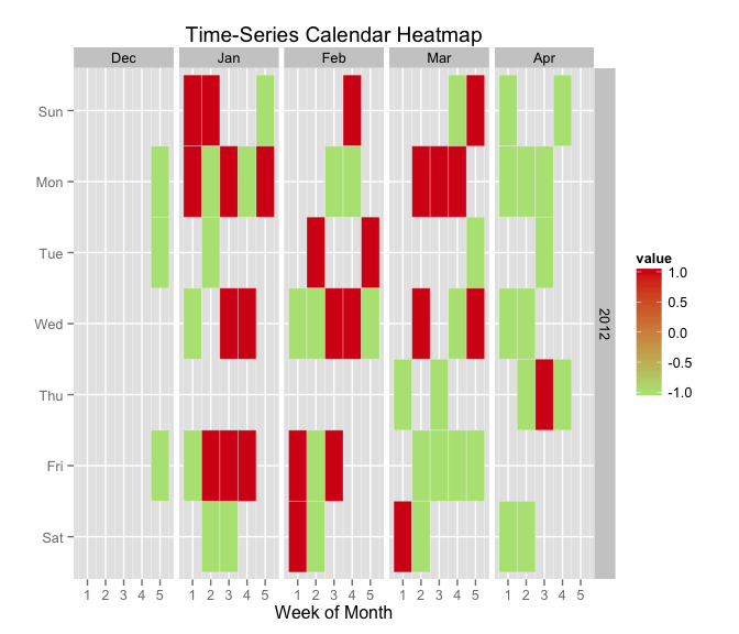
One interesting note here, the Bulls seem to have a lop sided margin they win by more that they lose. This would seem to indicate that they were a good team that year. The other thing to note is that there is a lot of orange meaning it's hard to tell whether they won or lost in all but the most extreme cases, like winning by 40. Thus it is hard to determine whether they are actually good team as far as wins and losses are concerned.

We can change this to show wins and losses opposed to the margin of victory.

# Binary win loss

final2 <- lapply(final, function(x) data.frame(date = x$date, win = ifelse(x$margin > 
    0, 1, -1)))

cal.heatMap(final2[["Chicago Bulls"]], "win")

This tells a lot more of the story, in the case of the 2011-2012 Chicago Bulls, they were always on top.

We can see what I set out to resolve, the Timberwolves practically fell apart in April winning only one game.

cal.heatMap(final2[["Minnesota Timberwolves"]], "win")

The Orlando Magic seemed to fall apart towards the end as well.

cal.heatMap(final2[["Orlando Magic"]], "win")

In hindsight since the calendar heat map aspect did not pan out so well there may be better ways to visualize this data. I do like that this demonstrates a fairly consistent aspect of any data science endeavour, to answer the question you started with you often have to change paths as you get further in. Data Science is dynamic, letting the data tell you what works and what doesn't will get you much farther. It also helps to have code and data that lets you change paths easily.

Future

I think it would be cool given data over more years to be able to pick seasons and also be able to compare teams or even look over teams for multiple years. That is starting to get away from the simple nature of manipulate and move more towards shiny or d3, which I may think of converting this into.

Reproducibility Made Easy

A lot of times I think the biggest hurdle to analyzing data and investigating something interesting is getting your hands on the data. You can look at my last post to find some basketball data and the steps needed to use it. Some of my interest there was based on how the season progresses. But after thinking about ranking things over time movies seemed to be a better fit. Thus my next hurdle was to try to find some data related to movies and particularly box office sales.

There are a few other issues I have wanted to explore recently as well. I have read a lot about on types of analysis people have done and what there results are. If the area is going to latch on to the term 'data science' I think one thing that needs to be addresed is verifiabilty and reproducablitly, which are potentially the same thing but for the purpose of completness I mention both. What I mean by these are that anybody can read about the data I am using, the hypothosis I am making, the analysis employed and the results found and be able to verify that I am not full of shit.

I hope to address the problem of making data available. Another thing I find hard is keeping data up to date, to really verify my findings you should be able to run the analysis on data that is relavent. It can go stale fairly quickly if some method is not put in place to automate the process of pulling new data. The last issue is how to allow other people to reproduce the work you did. I hope to tackle all of theses issues here, maybe some more than others though.

Collect Data

The first step of getting data is usually the hardest. This is usually the least documented as well. If you do get lucky and there is some data that you can use it is often lacking any detail as to how it was collected, when, from where and by whom. Thus any questions you have are simple forced assumptions you must make. In every data mining/data science project I've worked on this has been hard. Usually there are many hurdles you have to jump through making it a success to actually have data. Once you recieve the data it is NOT and will NEVER be in the form that would be most useful for your purpose. I have found that collecting it myself can sometimes be the easist way to get data. This way you know all of the assumptions behind it. This does require a lot of work though and I hope the inderlying processes around data will get better so tht this in not the case.

Below you can see the my initial attempt at trying to find some movie data. The data was collected from Box Office Mojo using the R XML package.

library(XML)
library(lubridate)
# This is useful for imported data.
options(stringsAsFactors = FALSE)

# Source where data comes from.  
site <- "http://www.boxofficemojo.com/daily/chart/?view=1day&sortdate=2013-03-15&p=.htm"

# Read data from that site.
siteData <- readHTMLTable(site)

# We need to investigate this to see what we really need. Looking at the site will helps as well.
# We need to take the tenth element in this list.
mList <- readHTMLTable(site)[[10]]
# We need to remove some of the leading and trailing rows as well.
mList <- mList[4:(nrow(mList) - 1), ]
# Give the fields names.
names(mList) <- c("td", "yd", "Name", "Stu", "Daily", "peru", 
                  "perd", "num", "Avg", "Gross", "Day")
# SHow a subset of the data.
mList[14:18, ]

##    td yd        Name    Stu    Daily  peru perd num  Avg        Gross Day
## 17 14 12  Life of Pi    Fox $328,783  +80% -17% 646 $509 $120,448,917 115
## 18 15 13     Quartet  Wein. $265,313  +72% -25% 688 $386  $14,162,205  64
## 19 16 14  Dark Skies W/Dim. $188,460  +45% -52% 703 $268  $16,290,971  22
## 20 17 15 Warm Bodies   LG/S $185,718  +72% -38% 659 $282  $64,196,628  43
## 21 18 18     Emperor  RAtt. $183,452 +119% -45% 311 $590   $1,586,515   8

Some cleaning was already done in removing the items from the list to just get the table with the movie data, as well as removing lines from that table that are just noise. We also had to clean the names up a bit. Much more cleaning is required though. As with any data project this will fall into the 80/20 ratio of 80% of your time is spent cleaning and transforming the data into a usebale format and twenty percent is spent in doing actual analysis. All the interesting algorithms and visualizations you can use on data are not applicable until the correct amount of cleaning has happened. I often think of this task as data wrangling and person who is skilled in this craft as a data ninja. I don't think I have ever seen a job post for a data ninja either, but the skill is crucial.

Please don't use the above code in any loop construct to pull more data as that could create a lot of stress on the sites server, it will also take a while, I don't want it to go away, and I have made a far easier method for you to get all of the data if you keeping. If you just want the data you can use the following in R.

require(devtools)

## Loading required package: devtools

install_github("chRonos", "darrkj", quiet = TRUE)

## Installing github repo(s) chRonos/master from darrkj

## Installing chRonos.zip from
## https://github.com/darrkj/chRonos/archive/master.zip

suppressPackageStartupMessages(library(chRonos))
data(mvData)

str(mvData)

## 'data.frame':    196252 obs. of  13 variables:
##  $ date    : Date, format: "2009-07-17" "2009-07-18" ...
##  $ td      : chr  "12" "14" "11" "11" ...
##  $ yd      : chr  "-" "12" "14" "11" ...
##  $ name    : chr  "(500) Days of Summer" "(500) Days of Summer" "(500) Days of Summer" "(500) Days of Summer" ...
##  $ studio  : chr  "FoxS" "FoxS" "FoxS" "FoxS" ...
##  $ daily   : num  263178 310203 261120 125900 141175 ...
##  $ peru    : num  NA 0.18 -0.16 -0.52 0.12 -0.04 0.01 2.65 0.26 -0.18 ...
##  $ perd    : num  NA NA NA NA NA NA NA 0.9 1.02 0.96 ...
##  $ Theaters: num  27 27 27 27 27 27 27 85 85 85 ...
##  $ Avg     : num  9747 11489 9671 4663 5229 ...
##  $ Gross   : num  263178 573381 834501 960401 1101576 ...
##  $ Day     : num  1 2 3 4 5 6 7 8 9 10 ...
##  $ weekday : Ord.factor w/ 7 levels "Sun"<"Mon"<"Tues"<..: 6 7 1 2 3 4 5 6 7 1 ...

Update Data

The next issue is data falling out of relavency. If you run the above I can gaurantee that the data you have will be atleast a week old. What does stale data mean? Think about opening your favorite weather resource and it is predicting that it will rain last Tuesday. Thats useless since it does not help you to plan for your outdoor excursion tomorrow, even worse if you know it did not rain last Tuesday, now your thoughts on this source are tainted. You need to keep data up to date and relavent.

I could probably make a method to have this data up to date for whenever you pull it. I think I may do that but for now I think this is better. Included in this package is a function called mojoRef(). This takes care of refreshing the data for you. If you run it you can see the new dates streaming in as the data is being pulled and cleaned to align with the current data frame. This can easily be appended to the rest of the data. If you wanted something to be autonomous you could add your own line to the function to ruturn nothing but overwrite the source data.

mvData <<- rbind(mvData, mojoRef())

mojoRef <- function() {
    library(chRonos)
    data(mvData)
    # Start from the day after that most recent day.
    start <- max(mvData$date) + 1
    # Remove this data.
    return(mojo(start))
}

newData <- mojoRef()

## [1] "2013-05-16"
## [1] "2013-05-17"
## [1] "2013-05-18"
## [1] "2013-05-19"
## [1] "2013-05-20"
## [1] "2013-05-21"

What is really happening here is that we isolated what data we want, how we want it cleaned, and how that all has to happen. This is really only able to happen once your data requirements have converged. I took some time for me to figure out exactly how I wanted the date stored and cleaned. Once the aquostion part was correct then I worried about refreshing it. Donald Knuth stated that premature optimization is the root of all evil. I agree but I have an equally valid statement, premature automation is the root of all headaches. Once you really know what you want and you have some need to consume new data in a specified manner then you can automate the extraction process.

Make Data Available

Above you saw how easy it was to get the data that I have made available on Github. I need to thank Hadley Wickham for his devtools package which makes the process to get the package easy, as well as the people at Github for making the storage location very accesable.

Data can be made available in other methods as well. Read my last post on basketball data to see another method employed elsewhere that made the aquisition stage easy on my part. Simply google open data and you will find a vast array of current info on this problem. If you do some work that you think is relavent you should try give others access to it. I am not saying give away trade secrets or anything. Make it open to your audience. This may be ironing out the process for your coworkers, creating internal documentation, or something similar to this post. You will know the frustrations of not doing so the first time you inherit a project where decsions where made based on some data but you have know way of validating that it still holds true. Have you ever heard of Concept Drift?

Reproducable

To make any analysis done on the data reproducable has been a nuance in the past. There are many papars out there that you just have to take the authers word. There are also cases where after the fact it has been shown that the results were faked, so we can't trust everyone. If we make ourselves accountable people can have no other course of action but to believe us. If not they cannot merely say somehting is false, if the process is repeatable and reproducable then they must redo your work and show where it is not, and make sure their work is reproducable. Above I have shown just one manner in which you can make data accesable, but in that process I have also given all of the code to do these things, tried to explain what I was doing and why. I will leave you with a small sample of analysis which I hope my next post will go into more depth.

# Get rid of really old data.
mov <- mvData[year(mvData$date) > 2002, ]
# Movies that have a first day.
wholeMov <- unique(mov[mov$Day == 1, ]$name)
# Create a list of movies in this set.
mov <- mov[mov$name %in% wholeMov, ]

library(ggplot2)
# Lets look at one movie.
title <- "X-Men: First Class"
movie <- mov[mov$name == title, ]
qplot(Day, daily, data = movie, main = title)

# Zoom in on area of interest.
qplot(Day, daily, data = movie[1:40, ], main = title)

# The day of the week seems to have a big impact on sales.  Lets break it
# out into a plot for each day.
ggplot(movie, aes(Day, daily)) + geom_point() + facet_grid(. ~ weekday)

Getting Side-tracked with Basketball Data

The NBA playoffs are here. Recently I have been interested in analyzing sports data. I was able to find some NBA data from older seasons to be the most accessible. This is the data that I used. The code below will take care of downloading and importing it for you though. To start with I was not really sure what I wanted to look at, I just think its interesting exploring new types of data in diverse areas. This set is pretty interesting in that it has a lot of shot data, who, when, the result and most interesting, where. It has the x and y coordinates of every shot. I thought it would be cool to look at hot spots of field goals. First though we need to pull the data.

# Load packages used.
library(rbenchmark)
library(plyr)

# This is useful for importing data.
options(stringsAsFactors = FALSE)

# Create dir for data files.
dir <- "BBdata"
dir.create(dir, showWarnings = FALSE)
temp <- tempfile()

# Location of the files.
url1 <- "http://www.basketballgeek.com/downloads/2008-2009.regular_season.zip"

# Take the base of the file name at this loaction.
file <- basename(url1)

# Download the file from the internet.
download.file(url1, file)

# Extract zipped contents to directory.
unzip(file, exdir = dir)

# The list of unzipped files.
fileList <- list.files(dir)

# Only the csv data files.
fileList <- fileList[grep(pattern = "csv", x = fileList)]

# Full location to the files.
fileList <- paste(dir, fileList, sep = "/")

Method 1: rbind

I want to explore this data as a whole season so it all needs to be loaded into the workspace. The zip files come with a csv file for each game played in a season though. I tried to load each file and append it to a growing data set. I knew this would be slow but I was in no rush. I was not aware that it would take as long as it did though. You will see later just how slow. I then thought I could for the best way to do this.

The first method I tried was to simply read each file in and append it to a data frame. This is the easist solution. Wrapping this in a function is just used for benchmarking and profiling, it is an easy way to take imperative line by line instructions and call them without copy and paste later.

# Method which uses naive appending via rbind.
M1 <- function() {
    # Use rbind to append each file to the first.
    games <- read.csv(files[1], na.strings = "")
    # Drop first that was already loaded.
    file <- files[-1]
    # Loop over each file and append it to growing list.
    for (i in file) {
        tmpGame <- read.csv(i, na.strings = "")
        games <- rbind(games, tmpGame)
    }
    return(games)
}
files <- fileList[1:100]
system.time(games1 <- M1())[3]

## elapsed 
##   8.429

Method 2: preallocation

This method is pretty bad. I may want to pull more seasons that just 2008-2009 which will make it even worse. Most everywhere you look in relation to making something in R work faster you see vectorization for math operations and pre-allocation for data storage operations. Let’s see how much these methods help with the task at hand.

First though I want to create a useful function for initializing a data frame. This is a very handy function that I made and can clean up the look of preallocation when dealing with wide data frames. You don't have to be as verbose with listing out every variable. You can just give it a list of names and a number of rows and you have all of the preallocation taken care of.

initDF <- function(name, row) {
    # String which start the data frame istantiation.
    init <- "df <- data.frame("
    for (i in name) {
        init <- paste(init, i, " = rep(NA, ", row, "), ", sep = "")
    }
    init <- substr(init, 1, nchar(init) - 2)
    init <- paste(init, ")", sep = "")
    eval(parse(text = init))
    return(df)
}

# Method which uses preallocation.
M2 <- function() {
    # Read first file to get names in the data.
    game <- read.csv(files[1], na.strings = "")
    # The number of rows in the data.
    rows <- nrow(game)
    # Its hard to know this exactly before hand so be conservative with guess.
    estRows <- ceiling(rows * length(files) * 1.2)
    # Preallocate the data frame.
    games <- initDF(names(game), estRows)
    # Initialize index.
    j <- 1
    # Loop over each file.
    for (i in files) {
        game <- read.csv(i, na.strings = "")
        # How many rows are in this data set.
        len <- nrow(game)
        # Insert these rows into there spots in the preallocated data frame.
        games[j:(j + len - 1), ] <- game
        # Increment the index
        j <- j + len
    }
    # Remove the excess from our conservative guess.
    games <- games[1:(j - 1), ]
    return(games)
}
files <- fileList[1:100]
system.time(games2 <- M2())[3]

## elapsed 
##   6.227

The first thing I notice here is that I have to make a guess on the size of the data, which may not always be easy. Here I could use the results from the first method since I have already seen how many rows we will have. To make it more realistic I used an approximation and applied a fudge factor. The next problem is the code is odd in respect to the hoops you jump through to index correctly, to not overwrite old data or leave gaps in between appended sets. We did save some time though, not much but it does go faster. Was it worth it though, dealing with the indexing maze in order to gain a small speed improvement?

Method 3: do.call rbind

It appears there has been some discussion about this type of data wrangling. There is a better way to use rbind, via do.call. http://r.789695.n4.nabble.com/Concatenating-data-frame-td799749.html This gives me another method to look into. This calls rbind on the entire list in a vectorized manner instead of multiple times. We also get rid of all of the indexing mess.

# Method which uses do.call, rbind all at once.
M3 <- function() {
    # Initialize list that will store each loaded file.
    g <- vector("list", length(files))
    # Initialize the index.
    j <- 1
    # Loop over all of the files.
    for (i in files) {
        g[[j]] <- read.csv(i, na.strings = "")
        j <- j + 1
    }
    games <- do.call("rbind", g)
    return(games)
}
files <- fileList[1:100]
system.time(games3 <- M3())[3]

## elapsed 
##   1.228

Method 4: plyr's rbind.fill

Two things to note about the code itself; the size has reduced from the pre-allocation method and we have no indices to maintain. But the best outcome is the speed, a good improvement. I could probably live with this approach but I am intrigued by another similar post and its recommendation to use rbind.fill from the plyr package. http://r.789695.n4.nabble.com/Fast-dependable-way-to-quot-stack-together-quot-data-frames-from-a-list-td2532293.html I have used this in the past when I have sets which may have different columns as it provides a nice feature of imputing them to missing instead of the error received from the regular rbind. Let’s give this a try.

# Method which uses plyr, references say it is the fastest approach.
M4 <- function() {
    # Initialize list that will store each loaded file.
    g <- vector("list", length(files))
    # Initialize the index.
    j <- 1
    # Loop over all of the files.
    for (i in files) {
        g[[j]] <- read.csv(i, na.strings = "")
        j <- j + 1
    }
    games <- rbind.fill(g)
    return(games)
}
files <- fileList[1:100]
system.time(games4 <- M4())[3]

## elapsed 
##    1.43

The code is still pretty clean, we basically just replaced one line. For the case of only looking at the first 100 files it appears to be a little slower. Let's try each method on a larger set. We should also check that everything is working as we expect it to.

Comparison

# Time the first 200
files <- fileList[1:200]

# Run a side by side comparison of each method.
benchmark(replications = rep(1, 1), M1(), M2(), M3(), M4(), columns = c("test", 
    "replications", "elapsed"))

##   test replications elapsed
## 1 M1()            1  21.349
## 2 M2()            1  12.610
## 3 M3()            1   3.274
## 4 M4()            1   3.599

# Check that each method works.
all(all(games1 == games2, na.rm = TRUE), all(games2 == games3, na.rm = TRUE), 
    all(games3 == games4, na.rm = TRUE))

## [1] TRUE

Method 5: Recursion

Thinking through what is happening here leaves me wondering if all of these methods are bad. In the cases where we use indexing we are getting beat up by the copy on modify, every time we add new rows we copy the whole data frame due to immutability. The naive rbind approach is always looking for larger sections of contiguous memory and transporting everything there. Thus in the beginning it is small, copying every increasing sets around just keeps building up though. The do.call and rbind.fill method seem to closer to the pre-allocation time, I want to see what they are doing under the hood though before I say anything about them. I would imagine that a divide and conquer approach would work better here knowing where some of the sluggishness comes from. We can use the naive rbind but never have to carry the whole data frame, actually only half one time, a quarter twice and so on. R deals with recursion by adding the environment to the call stack. In a normal function you don’t worry about cleaning the local environment before you leave it because it will be destroyed when only moving the return object. In the case of recursion though we add the whole environment to the stack then jump to the next iteration. Do to the log nature of the divide and conquer we don't have to worry about going infinitely deep but we do have to worry about copying a lot of useless data at every new level of depth. Let’s clean the environment except what we actually care about.

# Recursive row binding, you don't carry huge sets around, has divide and
# conquer on memory usage, large set only appear at the top level of the
# recursion.
recurBind <- function(dList) {
    len <- length(dList)/2
    # Preallocate list for small improvement.
    data <- vector("list", len)
    j <- 1
    for (i in seq(len)) {
        # Merge each set of two sequential data sets together.
        data[[j]] <- rbind(dList[[(i * 2) - 1]], dList[[i * 2]])
        j <- j + 1
    }
    # In case length was odd, just add last set to the end.
    if (floor(len) != len) {
        data[[j]] <- dList[[len * 2]]
    }
    # Less data to store on the stack, tail call optimization would be nice
    # here.
    rm(dList, len, j)
    # Recursive call.
    if (length(data) > 1) {
        data <- recurBind(data)
    }
    return(data)
}

# Apply the recursive method.
M5 <- function() {
    # Initialize list that will store each loaded file.
    g <- vector("list", length(files))
    # Initialize the index.
    j <- 1
    # Loop over all of the files.
    for (i in files) {
        g[[j]] <- read.csv(i, na.strings = "")
        j <- j + 1
    }
    games <- recurBind(g)[[1]]
    return(games)
}
files <- fileList[1:100]
system.time(games5 <- M5())[3]

## elapsed 
##   1.049

It's faster than all the other methods, but I was actually thinking that it would be slower for this small case and would only be asymptotically faster once we take the rest of the files into consideration. Let's run the above test again and see how good it fares.

Comparison 2

# Time the first 500
files <- fileList[1:500]

# Run a side by side comparison of each method.
benchmark(replications = rep(1, 1), M1(), M2(), M3(), M4(), M5(), columns = c("test", 
    "replications", "elapsed"))

##   test replications elapsed
## 1 M1()            1  125.85
## 2 M2()            1   79.57
## 3 M3()            1   16.13
## 4 M4()            1   19.63
## 5 M5()            1    6.49

# Check that each method works.
all(games1 == games5, na.rm = TRUE)

## [1] TRUE

It seems I was right. The first two methods are performing very poorly. We can safely ignore them from here on out. To me this is a very interesting result; we used in what in reality is the slowest approach possible, rbind, in a clever manner to get the fastest approach. What if we apply some of the faster methods inside the recursion, or even get rid of the recursion altogether by smart looping in a manner that is equivalent to recursion but never has to recreate the local environment recursively. Is there a way that we can mimic tail call optimization or even compile this? I am sure there are even faster ways of doing this.

Basketball Analysis

What was all of this for again, oh yeah Basketball.

files <- fileList
games <- M5()
made <- games[, c("team", "player", "etype", "result", "x", "y")]
made <- made[made$etype == "shot", ]
made <- made[made$result == "made", ]
made <- made[, c("result", "x", "y")]
made <- made[complete.cases(made), ]
made$result <- ifelse(made$result == "made", 1, 0)
x <- tapply(made$result, made[, c("x", "y")], sum)
x <- ifelse(is.na(x), 0, x)
image(log(x), col = rainbow(30))

missed <- games[, c("team", "player", "etype", "result", "x", "y")]
missed <- missed[missed$etype == "shot", ]
missed <- missed[missed$result == "missed", ]
missed <- missed[, c("result", "x", "y")]
missed <- missed[complete.cases(missed), ]
missed$result <- ifelse(missed$result == "missed", 1, 0)
y <- tapply(missed$result, missed[, c("x", "y")], sum)
y <- ifelse(is.na(y), 0, x)
image(log(y), col = rainbow(30))

This code is pretty gross, it is more or less hacking to get a few plots, I realized I became so interested in importing the data in a fast and clean manner that I had little time to do anything with the actual data. At a first glance thought I expected to see the first chart but the second has me a little stumped. Maybe I will have time to look more into this later.

Does it Scale

Just to check how good this is lets run a few years. This adds the prior season.

# Data for the year prior.
url2 <- "http://www.basketballgeek.com/downloads/2007-2008.regular_season.zip"

# Take the base of the file name at this loaction.
file2 <- basename(url2)

# Download the file from the internet.
download.file(url2, file2)

# Extract zipped contents to directory.
unzip(file2, exdir = dir)

# The list of unzipped files.
newList <- list.files(dir)

# Only the csv data files.
newList <- newList[grep(pattern = "csv", x = newList)]

# Full location to the files.
newList <- paste(dir, newList, sep = "/")

length(newList)

## [1] 2359

# Time larger set
files <- newList
benchmark(replications = rep(1, 1), M3(), M4(), M5(), 
          columns = c("test", "replications", "elapsed"))

##   test replications elapsed
## 1 M3()            1  360.35
## 2 M4()            1  474.80
## 3 M5()            1   57.55